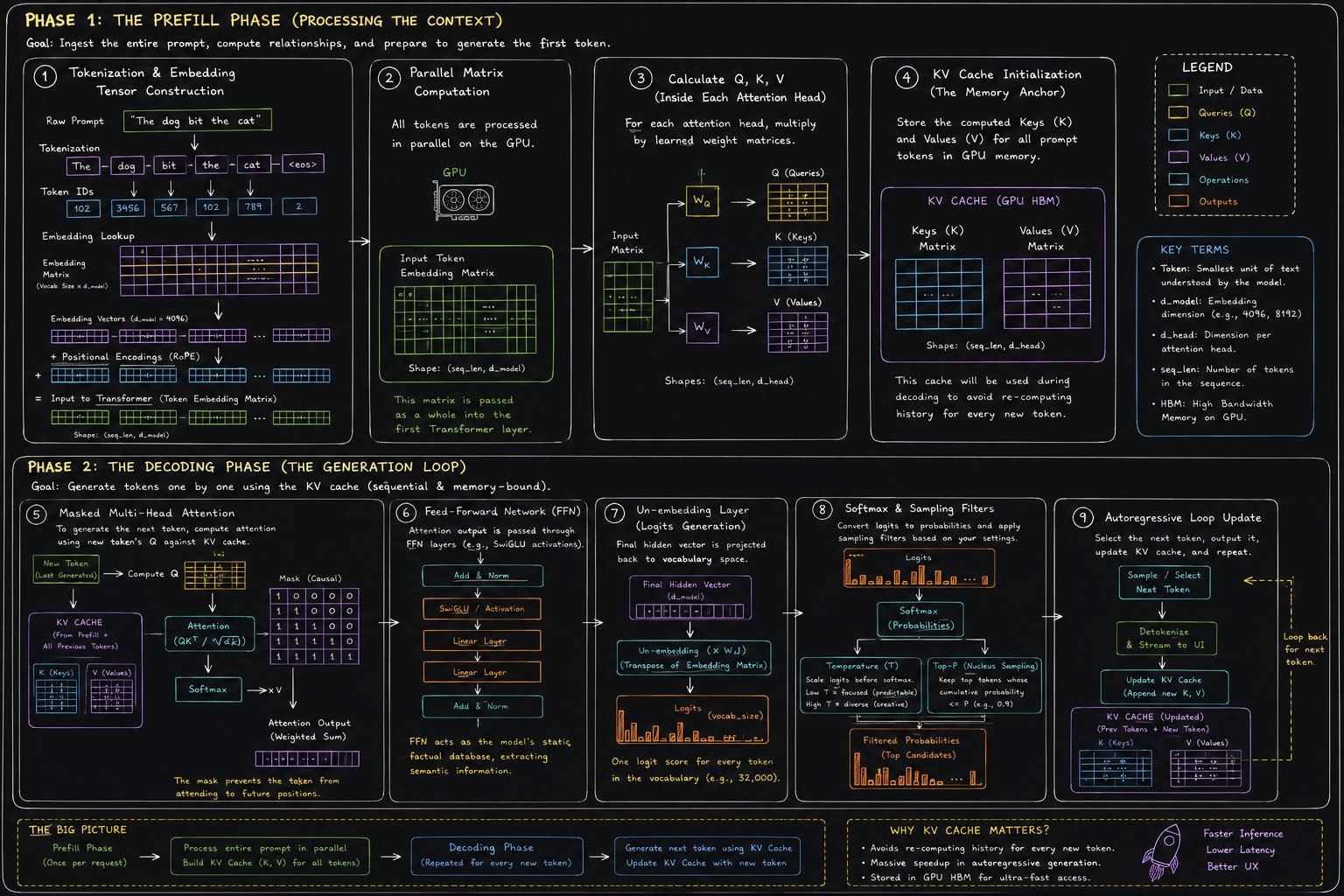
To truly understand Large Language Model (LLM) inferencing at a deep technical level, we must look past the simple abstraction of “predicting the next word”. Inferencing is a highly coordinated sequence of matrix multiplications, memory lookups, and hardware-level optimizations.
When you submit a prompt to an LLM, the inference engine executes 2 distinct phases: the Prefill Phase and the Decoding Phase.
Phase 1: The Prefill Phase (Processing the Context)
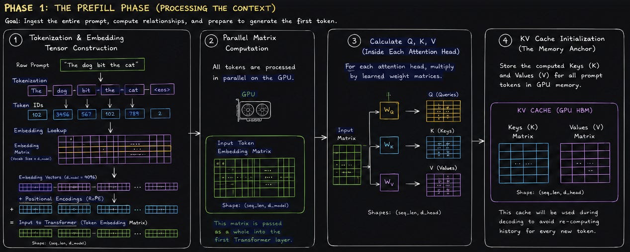
The prefill phase occurs the instant you hit “Send”. Its objective is to ingest your entire prompt, calculate the semantic relationships between all your input words, and prepare the model to write the first token of its response.
Step 1: Tokenization and Embedding Tensor Construction
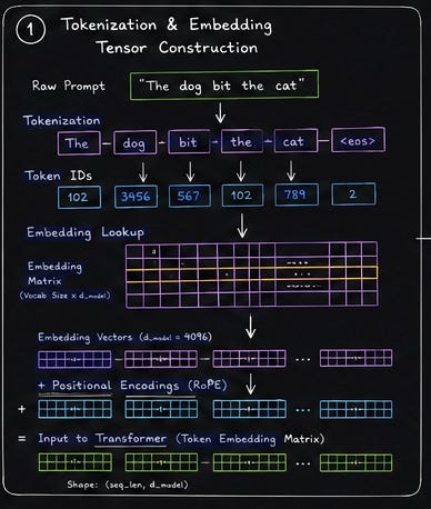
Your raw text prompt is split into standard units called tokens. Each token corresponds to a specific ID inside the model’s vocabulary matrix.
These token IDs are looked up in a massive weight matrix known as the Embedding Layer.
The embedding layer converts each token ID into a dense mathematical vector of continuous numbers (often 4096 or 8192 dimensions deep).
Positional Encodings are mathematically added directly using these vectors. This ensures the model retains structural context, understanding the exact difference between “The dog bit the cat” and the “The cat bit the dog”.
Step 2: Parallel Matrix Computation
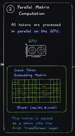
Unlike the output phase, the prefill phase is highly parallelized. Because the entire prompt is available upfront, the graphics processing unit (GPU) processes all input tokens simultaneously. The sequence of embedding vectors is passed into the first Transformer layer as a single massive matrix
Step 3: Calculating Queries, Keys, and Values (Q,K,V)
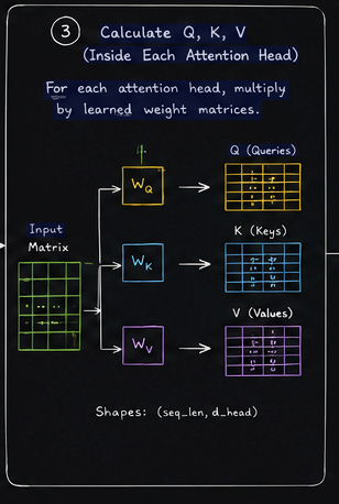
Inside every attention head of Transformer layer, the token matrix is multiplied by 3 distinct learned weight matrices to produce 3 new matrices:
Queries (Q): What a token is actively searching for in the rest of the sentence
Keys (K): What information a token contains that might be relevant to other tokens.
Values (V): The actual semantic content of the token.
Step 4: The KV Cache Initialization (The Memory Anchor)
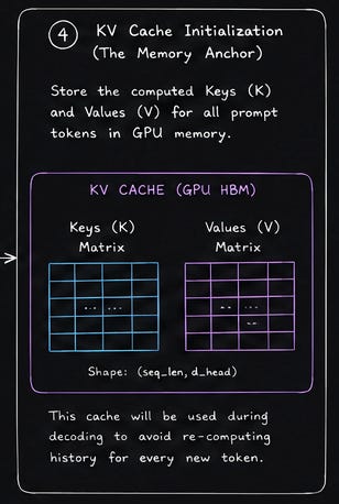
This is the single most critical performance optimization in modern LLM inferencing. During the prefill phase, the calculated Key (K) and Value (V) matrices for all your prompt tokens are computed once and stored directly inside the GPU’s high-bandwidth memory. This storage space is called the KV Cache. By saving these values now, the model avoids recalculating the historical context for every single word it generates later.
Phase 2: The Decoding Phase (The Generation Loop)
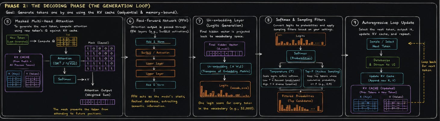
Step 5: Masked Multi-Head Attention
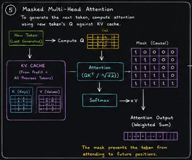
To generate the very first new token, the model executes the standard self-attention equation across the Q,K and V matrices:
However, during this phase, the attention mechanism is masked. Because it is generating text chronologically, a token is mathematically forbidden from looking at any information that supposedly comes after it. It can only compute scores against the historical tokens stored inside the KV Cache.
Step 6: The Feed-Forward Network Processing
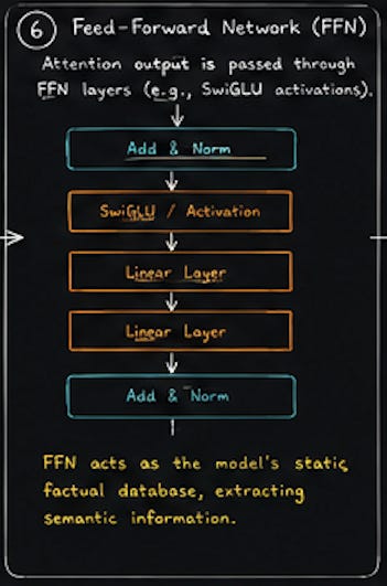
The output matrix from attention mechanism is passed through a sequence of Feed-Forward Network layers. While the attention layers are designed to map the spatial relationships between tokens, the FFN layer acts as the model’s static factual database, extracting semantic facts based on the mapped context.
Step 7: The Un-embedding Layer
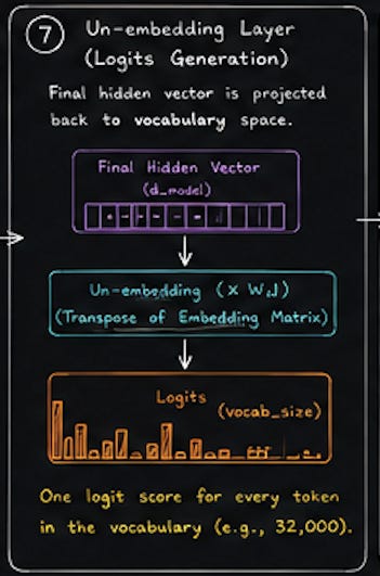
The final hidden vector emerging from the last Transformer layer represents the mathematical essence of the next token. To translate this back into vocabulary words, it is multiplied by the inverse of the embedding matrix (the un-embedding layer).
This operation outputs a sequence of raw numerical values called logits.
There is exactly one logit score for every single word/token in the model’s dictionary.
Step 8: Softmax Transformation and Sampling Filters
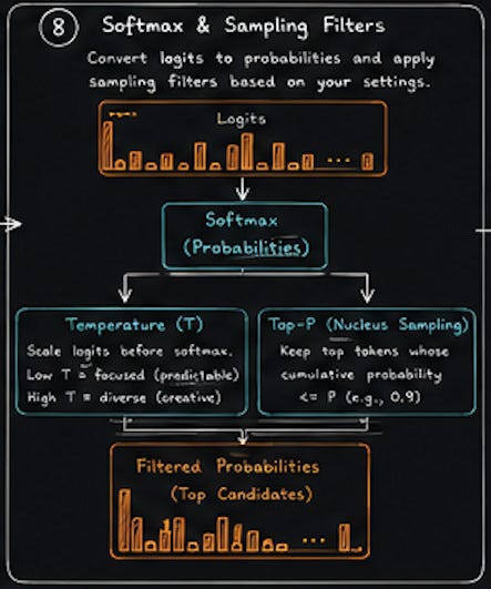
The raw logits are passed through a Softmax function to turn them into clean percentages. If your model vocabulary is 32,000 words, you now have 32,000 distinct probability scores that altogether sum up to 1.0. The inference engine then applies your generation parameters:
Temperature: Divides the logits before Softmax. A lower temperature crushes lower-probability options, rendering the model predictable. A higher temperature flattens the distribution, raising the probability of unusual word choices.
Top-P (Nucleus Sampling): Sorts the tokens by probability and discards everything outside the top cumulative percentage pool (e.g., the top 90% of probability weight), eliminating chaotic outliers entirely.
Step 9: Autoregressive Loop Update
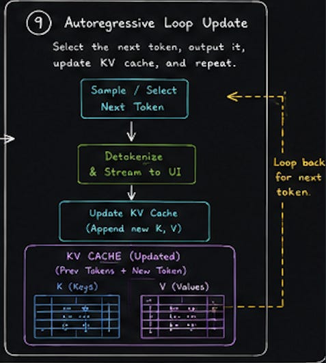
The final winning token is selected, converted back into text via the de-tokenizer, and streamed to your user interface. Crucially, the Key and Value matrices for this brand-new token are calculated and immediately appended to the existing KV Cache. The model then restarts Phase 2, feeding only this single new token back into the input layer while referencing the expanded KV cache for historical memory.
The complete diagram is shown below: